
TL;DR: When queries are slow, indexes are here to help. Postgres supports a variety of index types, including multi-column and partial indexes, as well as more complex ones like indexes on expressions. However, growing the number of indexes to optimize query performance comes with a massive caveat: storage cost. A feature many people don’t know about: extended statistics. These extended statistics can help to improve query plans while their storage usage is almost non-existent.
If you spend enough time staring at bad query plans, you see a very common pattern. Postgres is choosing a bad plan. Not because it is careless or because it is trying the easiest thing, but because it is a perfectly rational choice given its completely wrong picture of the data.
The problem is typically row estimation or data cardinality.
When several predicates are correlated, PostgreSQL’s default per-column statistics can give the query planner a misleading view of how many rows will survive a filter. Once an estimate is wrong, everything downstream gets shaky: join order, join method, parallelism, hash sizing, sort strategy, spill risk, everything. This is where extended statistics come in.
When I started this blog post, I was aware of extended statistics, but never really used them myself. Now, I’m annoyed at myself. I should have. Much earlier. Would have saved gigabytes of indexes. Let me show you why.
The Short Version
Create Statistics lets Postgres collect additional statistics that ordinary per-column statistics cannot really represent.
In practice, there are four specific types of queries that can be optimized by extended statistics:
- Correlated predicates filter multiple columns with dependencies among them.
- Multi-column distinct counts provide cardinality information about multiple columns.
- Issues with skewed value combinations where one cluster is larger than the other.
- Data unpacked via expressions, which doesn’t have an index on expressions.
In terms of code, these come down to two common forms:
–-- Alternative to index on expressions CREATE STATISTICS stats_expr ON (date_trunc(‘day’, created_at)) FROM events; --- What people normally mean by --- extended statistics CREATE STATISTICS stats_multi (dependencies, ndistinct, mcv) ON plan_tier, region, billing_status FROM tenants; |
The first single-expression enables Postgres to understand what’s really inside the data. It’s a much cheaper alternative to indexes on expressions. Removing the write overhead and improving the query plan. One great use-case is JSONB path extraction.
The second multi-column form is what most people think of when talking about extended statistics.
As you can see, there are three types of extended statistics we can create:
- With dependencies, we define the strong dependency between columns.
- For distinct values, ndistinct provides Postgres with better estimates about how many distinct multi-column combinations actually exist.
- And mcv helps when certain combinations are typically unlikely, or effectively impossible.
Omitting the definition, Postgres collects all supported multivariate kinds for the given statistics object.
Remember, just like normal statistics, CREATE STATISTICS just defines the statistics collection. ANALYZE is still the command that collects and materializes statistics.
Why Extended Statistics?
Whenever you create a table and store data, Postgres creates statistics that enable the query planner to make decisions about the “optimal” execution plan for a specific query. However, by default, those statistics are mostly per-column. This works great until your query depends on relationships between multiple columns.
Suppose you have a query with the following where-clause.
WHERE plan_tier = 'enterprise' AND region = 'eu-central' AND billing_status = 'active' |
In real production data, such columns are often correlated.
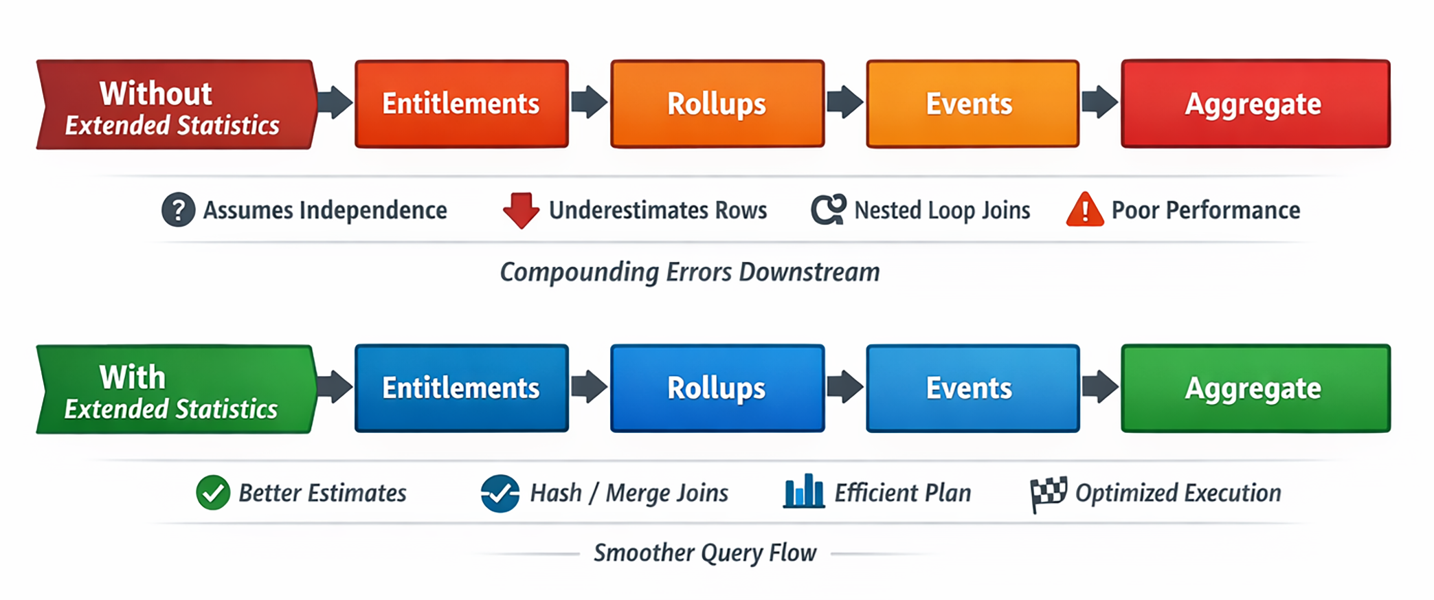
But without extended statistics, PostgreSQL tends to behave as if each predicate reduces the row set independently. That gives you row estimates that look mathematically tidy and operationally ridiculous. And the issues stack.
First, PostgreSQL underestimates the number of filtered tenants. Then it underestimates the number of entitlements those tenants have. Finally, it underestimates how many rollup rows and event rows fan out from there.
By the time it reaches a large join or aggregate, the plan can be off by one or two orders of magnitude.
The planner is not failing because it cannot compare nested loops with hash joins. It is failing because it is comparing them with the wrong estimated input sizes.
That distinction matters. If the row estimates are wrong, the planning cost becomes a guessing game.
The Default Postgres Knowledge
With every ANALYZE, PostgreSQL stores per-column stats in pg_statistics. These statistics include information on null fractions, the number of distinct values, common histogram bounds, most common values and frequencies, and more. All important information, but limited to column-local information.
With single-column filters, such as col = constant or col BETWEEN ..., Postgres does really well. The problem starts with queries that need joint distribution.
Suppose a table has one million rows with the following distribution:
plan_tier = 'enterprise'matches 6% of the rowsregion = 'eu-central'matches 25% of the rows- and
billing_status = 'active'matches 80% of the rows
Without extended multi-column statistics, Postgres assumes full independence of the rows:
1,000,000 * 0.06 * 0.25 * 0.80 = 12,000 rows |
In the real world, those columns aren’t independent, though. Depending on our query, two or more columns are interconnected. Hence, the real answer may be 40,000 rows. Maybe it’s 60,000 rows. Maybe it’s just 5,000 rows. We don’t know. Per-column statistics alone cannot answer that question.
Assuming independence is not a bug in Postgres. It’s a missing fact about the data, and extended statistics fill in the blanks.
Benchmarking Extended Statistics
To provide concrete evidence, I built a synthetic but intentionally realistic SaaS analytics workload with four tables: tenants, tenant_entitlements, usage_rollups, and analytics_events.
The data set was shaped specifically to expose the planner’s blind spots when it comes to:
- The correlation between
plan_tier,region, andbilling_status. - Premium entitlements are concentrated in enterprise tenants and feature activity.
(tenant, feature, day)combinations in rollups aren’t random.
In other words, exactly the kind of workload where simple-column statistics tend to lie harshly in your face.
It’s important to remember that this dataset is synthetic. But, synthetic in the same sense that a wind tunnel is synthetic. It is controlled in order to isolate a real phenomenon.
Isolating The Problem With Data Shapes
Each table was designed to surface a specific planner weakness with single-column statistics.
Table: tenants
The tenant segmentation columns are correlated in a way that SaaS production data often is. Enterprise tenants are not evenly distributed across regions, and billing status is not independent of plan tier.
If PostgreSQL treats those filters as independent, it immediately misestimates the qualifying tenant population.
Table: tenant_entitlements
Premium features such as sso, audit_logs, and workflows are much more common in enterprise tenants than in lower tiers.
That matters because once you filter to enterprise tenants, the entitlement predicate is no longer an ordinary reduction over a random population. It is another correlated slice layered atop the first.
Table: usage_rollups
This table creates a realistic time-bounded fanout. Each tenant-feature pair can contribute multiple daily rollup rows in the last 30 days, and that distribution is not uniform.
That gives the planner a real multi-dimensional selectivity problem around (tenant_id, feature_name, rollup_day).
Table: analytics_events
This is the explosive fact table. For each qualifying tenant-feature pair, there can be many raw event rows, especially for hot feature/event-type combinations.
That is what makes a bad tenant estimate so dangerous: once PostgreSQL is wrong at the top of the plan, the downstream fanout gets much worse.
Skew was deliberate, too. A handful of feature combinations were made especially hot because smooth distributions are not where planners usually suffer most. Trouble starts when a few combinations dominate the workload, and independence assumptions blur them into a fake average world.
The Reporting Query
Now, let’s see our query. In this example, we ask a simple business question: “Among active enterprise tenants in one important region, which premium features generated the most recent activity?”
SELECT e.feature_name, count(*) AS total_events, sum(r.request_count) AS rolled_requests FROM tenants t JOIN tenant_entitlements te ON te.tenant_id = t.id JOIN usage_rollups r ON r.tenant_id = t.id AND r.feature_name = te.entitlement JOIN analytics_events e ON e.tenant_id = t.id AND e.feature_name = r.feature_name WHERE t.plan_tier = 'enterprise' AND t.region = 'eu-central' AND t.billing_status = 'active' AND te.entitlement IN ('sso', 'audit_logs') AND r.rollup_day >= CURRENT_DATE - 30 AND e.event_type IN ('view', 'click', 'run') GROUP BY e.feature_name ORDER BY rolled_requests DESC; |
For a full overview across multiple regions, we run a similar, slightly extended version that uses a common table expression and a final aggregation step per region.
WITH regional_feature_totals AS ( SELECT t.region, e.feature_name, count(*) AS total_events, sum(r.request_count) AS rolled_requests FROM tenants t JOIN tenant_entitlements te ON te.tenant_id = t.id JOIN usage_rollups r ON r.tenant_id = t.id AND r.feature_name = te.entitlement JOIN analytics_events e ON e.tenant_id = t.id AND e.feature_name = r.feature_name WHERE t.plan_tier = 'enterprise' AND t.billing_status = 'active' AND t.region IN ('eu-central', 'ap-southeast', 'us-east') AND te.entitlement IN ('sso', 'audit_logs', 'workflows') AND r.rollup_day >= CURRENT_DATE - 30 AND e.event_type IN ('view', 'click', 'run') GROUP BY t.region, e.feature_name ) SELECT region, feature_name, total_events, rolled_requests FROM ( SELECT region, feature_name, total_events, rolled_requests, row_number() OVER ( PARTITION BY region ORDER BY rolled_requests DESC, total_events DESC, feature_name ) AS regional_rank FROM regional_feature_totals ) ranked WHERE regional_rank <= 3 ORDER BY region, regional_rank; |
Both queries have the same basic shape:
- Define a tenant slice
- Restrict to entitled features
- Join recent rollups
- Expand into raw events
- Aggregate back down
- Rank by region in the multi-region case
The critical part is that the final output is small, but the intermediate join graph is not.
That makes these queries easy for humans to underestimate and easy for PostgreSQL to mishandle if its row estimates are wrong.
Breaking Down The Query Shape
Before looking at plans, it is worth breaking the benchmark SQL into conceptual stages. This is useful because the whole point of CREATE STATISTICS is to improve the planner’s understanding of how many rows flow from one stage into the next.
If the above queries make sense to you, jump to the next section. Otherwise, keep reading. We’ll break them down bit by bit.
Stage 1: Define The Tenant Slice
Both benchmark queries start by defining a tenant population.
For the single-region query, the slice is:
WHERE t.plan_tier = 'enterprise' AND t.region = 'eu-central' AND t.billing_status = 'active' |
For the multi-region query, we extend the slice with multiple regions.
WHERE t.plan_tier = 'enterprise' AND t.billing_status = 'active' AND t.region IN ('eu-central', 'ap-southeast', 'us-east') |
This first step is deceptively important. It establishes the base cardinality for everything downstream. If PostgreSQL gets this wrong, every later fanout estimate is built on the wrong tenant population.
This is also the stage where dependencies and mcv matter most. PostgreSQL needs to know whether this is a tiny, very selective slice or a larger, hotter cohort than independent selectivities would suggest. We’ll get deeper into the different types of statistics in a few.
Stage 2: Filter By Tenant Entitlement
The next logical stage is feature eligibility combined with entitlements:
JOIN tenant_entitlements te ON te.tenant_id = t.id ... AND te.entitlements IN (...) |
This is more subtle than a normal dimension join. It is not merely saying "bring in some metadata." It is saying "only keep features the tenant is actually licensed to use, and only for a selected premium subset."
That means the entitlement table acts as both a join target and a correlated feature filter.
This is one reason the query behaves more like a real SaaS analytics workload than a toy star-schema aggregation. Eligibility and usage are not independent concepts. They are linked.
Stage 3: Bind Recent Usage To The Eligible Features
The rollup join further narrows the universe.
JOIN usage_rollups r ON r.tenant_id = t.id AND r.feature_name = te.entitlement ... AND r.rollup_day >= CURRENT_DATE - 30 |
At this stage, the query is no longer operating on abstract tenants or abstract features. It is operating on recent, entitled, tenant-feature activity.
This is where the query starts to accumulate multiplicity:
- One tenant can have multiple matching entitlements.
- One tenant-feature pair can have multiple recent rollup days.
So the row count begins expanding before the large event table even arrives.
Stage 4: Expand To Raw Events
Then the query hits the event table. This is the high-cardinality explosion point.
JOIN analytics_events e ON e.tenant_id = t.id AND e.feature_name = r.feature_name ... AND e.event_type IN (...) |
Now, the planner must reason about how many raw events belong to the already filtered tenant-feature population. If Postgres still thinks it is working with a small intermediate result at this stage, nested loops and repeated index probes can look cheap when they are not.
This is why bad estimates often surface as obviously wrong join strategies only later in the plan. The root cause is upstream, but the pain becomes visible at the join with the large fact table.
Stage 5: Collapse The Explosion Back Into Something Small
Last, we group and order. The single-region query then does a full group and order.
GROUP BY e.feature_name ORDER BY rolled_requests DESC |
The multi-region queries only by groups inside the CTE, then later rank those grouped rows by region.
GROUP BY t.region, e.feature_name |
This stage is important because it makes the query look cheap if you only stare at the result set. The final output is tiny. However, the work to get there is not.
That is one of the reasons this reporting query is such a good demonstration of the planner. Human readers see two rows or a handful of ranked features and instinctively think "small result, small query." PostgreSQL has to survive the large intermediate join graph before it earns that small result.
Stage 6: Ranking In The Multi-Region Query
The multi-region query adds one more stage that the single-region query lacks.
row_number() OVER ( PARTITION BY region ORDER BY rolled_requests DESC, total_events DESC, feature_name ) AS regional_rank ... --- followed by WHERE regional_rank <= 3 |
This means the multi-region query is not only a join-and-aggregate problem. It is also a ranking problem. Once the grouped regional rows are produced, PostgreSQL still has to sort them in a partition-aware way and keep the top entries per region.
This is why the multi-region benchmark surfaces more temp I/O and more sort pressure. It broadens the tenant slice and adds a reporting-style ranking stage on top of the already expensive joins.
Extended Statistics To The Rescue
When we look at those issues, our first reaction is to add multi-column and partial indexes. If we want to be clever, we also add indexes on expressions to precompute some values (such as the day).
However, we’ll use three extended statistics to cover the main failure modes:
- Correlated tenants columns
- Tenant and entitlements combinations
- Rollup combinations
Let’s have a quick look at how we can use extended statistics to influence the query planner’s decision tree.
Remember, we have to run ANALYZE to calculate and fill the statistics after creation.
Type: dependencies
Functional dependency statistics help PostgreSQL determine that some columns predict others strongly enough that treating them as independent is incorrect.
Classic examples:
- Country strongly predicts currency
- State strongly predicts time zone
- The tenant segment strongly predicts entitlement families
In this report:
CREATE STATISTICS stats_tl_segment_dependencies (dependencies) ON id, plan_tier, region, billing_status FROM tenants; |
These are most useful for clauses like:
WHERE plan_tier = 'enterprise' AND region = 'eu-central' AND billing_status = 'active' |
This is the case where the second and third predicates do not reduce the row set nearly as much as the planner thinks. As a mental note, dependencies fixes “these filters are not independent.”
Type: mcv
MCV stands for most common values, but for extended statistics, the better mental model is most common combinations.
In the report:
CREATE STATISTICS stats_tl_segment_mcv (mcv) ON plan_tier, region, billing_status FROM tenants; |
This lets PostgreSQL learn things like:
('enterprise', 'eu-central', 'active')is especially common,('enterprise', 'ap-southeast', 'canceled')is rare,- and some combinations never occur at all.
That matters because many planner failures are not about smooth distributions. They are about skew. As a mental model, mcv fixes “this exact combination is hotter, colder, or more impossible than the averages suggest.”
Type: ndistinct
Finally, ndistinct tells PostgreSQL how many distinct combinations of columns exist, rather than how many distinct values each column has individually.
In the report, we actually use two ndistinct stats:
CREATE STATISTICS stats_tel_entitlement_ndistinct (ndistinct) ON tenant_id, entitlement FROM tenant_entitlements; CREATE STATISTICS stats_url_feature_ndistinct (ndistinct) ON tenant_id, feature_name, rollup_day FROM usage_rollups; |
These help PostgreSQL reason about questions such as:
- How many entitlements does a tenant typically have?
- How many recent rollup rows exist per
(tenant, feature)pair? - How many distinct
(tenant, feature, day)combinations survive a date filter?
That matters for group-by estimates, distinct counts, and downstream fanout. As a mental rule, ndistinct fixes “these grouped or joined combinations are not as numerous as the planner thinks.”
What PostgreSQL Stores
This is where it really gets interesting. We could solve all of the above issues with additional indexes. But indexes are expensive to keep up to date, and storage-wise.
Extended statistics, on the other hand, are fairly cheap. No complex tree structures to update, no massive WAL impact, almost none of the additionally required storage capacity.
Extended statistics definitions live in pg_statistic_ext, and the collected data lives in pg_statistic_ext_data.
pg_statistic_exttells you what objects exist.pg_statistic_ext_datatells you what data has actually been collected.
In this benchmark, the total storage footprint for the statistics objects was about 2,059 bytes. Broken down, it looks like:
- Tenant-Segment
mcv: ~1,049 bytes - Tenant-Segment
dependencies: ~518 bytes - Entitlement
ndistinct: ~220 bytes - Rollup
ndistinct: ~272 bytes
That is the whole point. These are not giant shadow indexes. They are planner metadata.
Their job is not to speed up lookups directly. Their job is to prevent PostgreSQL from hallucinating an incorrect data distribution. Postgres isn’t AI, hallucinating isn’t what it’s supposed to do 😆
Fixing Execution Plans!
When I started out with this blog post, my initial thought was to prove better plans with improved query times. While there was some improvement, it wasn’t to the extent I hoped for. But the estimates got much better. On larger data sets, you’ll definitely see improvements. That said, the most important result was not runtime. It was planner accuracy.
The scenarios:
| Scenario | Average Time | Worst Estimate | Additional Storage |
|---|---|---|---|
| Extended statistics | 2,857.896 ms | 48.27x | 2.0 KiB |
| Baseline + Composite Join-Key Indexes | 5,882.659 ms | 106.48x | 37.64 MiB |
| Baseline + Events (feature_name, event_type, tenant_id) | 4,781.551 ms | 108.7x | 31.45 MiB |
| Baseline + Partial Hot-Path Indexes | 4,765.351 ms | 106.22x | 30.20 MiB |
| Extended Statistics + Partial Hot-Path Indexes | 4,876.187 ms | 46.65x | 30.21 MiB |
Each query was run 5 times. You can find the full results (execution plans, runtime per iteration) in the repository.
Single-Region Query
The current schema uses single-column indexes as the common baseline. That leaves PostgreSQL enough access paths to avoid fully sequential execution, but it still has to estimate the intersection of correlated tenants, entitlements, rollups, and events predicates.
| Metric | Value |
|---|---|
| Average execution time | 14,168.174 ms |
| Average planning time | 4.134 ms |
| Execution samples | 31,093.955 ms, 29,065.788 ms, 3,564.811 ms, 3,570.114 ms, 3,546.200 ms |
| Planning samples | 5.058 ms, 3.952 ms, 8.969 ms, 1.899 ms, 0.793 ms |
| Join chain | Nested Loop:Inner -> Nested Loop:Inner -> Nested Loop:Inner |
| Scan nodes | Index Scan, Bitmap Heap Scan, Bitmap Index Scan, Index Scan, Index Scan |
| Top-level rows | 7 estimated / 2 actual |
| Worst estimate | Nested Loop: 178,389 estimated / 18,774,720 actual (105.25x) |
| Worst estimate path | Sort -> Aggregate -> Nested Loop |
With extended statistics, we were able to improve the query plan and save storage:
| Metric | Value |
|---|---|
| Average execution time | 2,857.896 ms |
| Average planning time | 3.025 ms |
| Execution samples | 4,318.854 ms, 2,612.261 ms, 2,396.848 ms, 2,467.702 ms, 2,493.816 ms |
| Planning samples | 6.719 ms, 2.067 ms, 2.128 ms, 2.243 ms, 1.970 ms |
| Join chain | Hash Join:Inner -> Nested Loop:Inner -> Merge Join:Inner |
| Scan nodes | Bitmap Heap Scan, Bitmap Index Scan, Bitmap Heap Scan, Bitmap Index Scan, Bitmap Heap Scan, Bitmap Index Scan, Index Scan |
| Top-level rows | 7 estimated / 2 actual |
| Worst estimate | Hash: 12,966 estimated / 625,824 actual (48.27x) |
| Worst estimate path | Sort -> Aggregate -> Gather Merge -> Sort -> Aggregate -> Hash Join -> Hash |
The planner stopped acting like it was dealing with a small joins and started acting like it understood there was real intermediate volume.
One subtle but important detail: the planner’s total estimated cost went up after extended statistics.
That is not a regression signal. It means PostgreSQL finally believed the query was more expensive than its earlier fantasy suggested.
A higher estimated cost with better row estimates can indicate a healthier planner model.
Multi-Region Query
For the more complex multi-region query, the execution time (on average) results were actually quite a bit faster.
Baseline:
| Metric | Value |
|---|---|
| Average execution time | 24,933.705 ms |
| Average planning time | 3.648 ms |
| Execution samples | 84,815.859 ms, 12,696.190 ms, 11,819.487 ms, 8,482.936 ms, 6,854.054 ms |
| Planning samples | 6.125 ms, 5.681 ms, 2.067 ms, 2.181 ms, 2.187 ms |
| Join chain | Merge Join:Inner -> Nested Loop:Inner -> Merge Join:Inner |
| Scan nodes | Subquery Scan, Bitmap Heap Scan, Bitmap Index Scan, Bitmap Heap Scan, Bitmap Index Scan, Bitmap Heap Scan, Bitmap Index Scan, Index Scan |
| Top-level rows | 28 estimated / 5 actual |
| Worst estimate | Sort: 53,580 estimated / 17,164,496 actual (320.35x) |
| Worst estimate path | Incremental Sort -> Subquery Scan -> WindowAgg -> Incremental Sort -> Aggregate -> Gather Merge -> Sort -> Aggregate -> Merge Join -> Sort |
With extended statistics in place:
| Metric | Value |
|---|---|
| Average execution time | 7,289.319 ms |
| Average planning time | 2.875 ms |
| Execution samples | 7503.924 ms, 8,261.715 ms, 7,433.035 ms, 8,181.565 ms, 5,066.357 ms |
| Planning samples | 9.244 ms, 0.932 ms, 1.039 ms, 1.801 ms, 1.359 ms |
| Join chain | Hash Join:Inner -> Nested Loop:Inner -> Merge Join:Inner |
| Scan nodes | Subquery Scan, Bitmap Heap Scan, Bitmap Index Scan, Bitmap Heap Scan, Bitmap Index Scan, Bitmap Heap Scan, Bitmap Index Scan, Index Scan |
| Top-level rows | 28 estimated / 5 actual |
| Worst estimate | Nested Loop: 68,387 estimated / 1,113,566 actual (16.28x) |
| Worst estimate path | Incremental Sort -> Subquery Scan -> WindowAgg -> Incremental Sort -> Aggregate -> Gather Merge -> Sort -> Aggregate -> Hash Join -> Hash -> Nested Loop |
That is not a minor refinement. That is PostgreSQL being dragged back into the same postal code as reality.
The query was still large, still spill-prone, still a real reporting workload. Extended statistics did not repeal the laws of physics. They just gave the planner a much better model of the data flowing through the plan.
Did it make the queries faster?
Sometimes yes, sometimes no. That is exactly why this topic is worth writing about carefully.
Single-Region Runtime
- Baseline average: 14,168.174 ms
- Extended statistics average: 2,857.896 ms
That looks spectacular until you inspect the samples:
(Run #1) 31,093.955 ms (Run #2) 29,065.788 ms (Run #3) 3,564.811 ms (Run #4) 3,570.114 ms (Run #5) 3,546.200 ms |
The baseline average was distorted by two extreme first runs. The top-level plan shape remained stable, suggesting cold-cache or warm-up effects rather than the planner randomly choosing different strategies.
So the obvious claim is not “extended statistics made this 5x faster.”
The claim is more like “extended statistics dramatically improved planner knowledge, and on this workload, that correlated with better steady-state behavior.”
Multi-Region Runtime
- Statistics-only: 7,289.319 ms
- Best index-only strategy: 6,886.473 ms
So the fastest measured scenario for the broader reporting query was not the statistics-only one.
That does not weaken the case for CREATE STATISTICS. It clarifies it.
Extended statistics improve cardinality estimates. They do not create new physical access paths. Indexes do.
Sometimes, a storage-heavy index strategy will beat a statistics-only strategy on runtime, even while the planner remains less accurate about the data.
Planning and execution are related problems, not identical ones.
Why The Index Comparison Matters
One of the more interesting results in the benchmark was that some index-heavy scenarios looked appealing in planner cost or runtime, while remaining much worse in estimation quality.
In both single- and multi-region cases, the difference in required storage for indexes and extended statistics is quite significant.
- Extended statistics: about 2.0 KiB
- Index-heavy alternatives: about 30.20 MiB to 37.64 MiB
That is the underrated part.
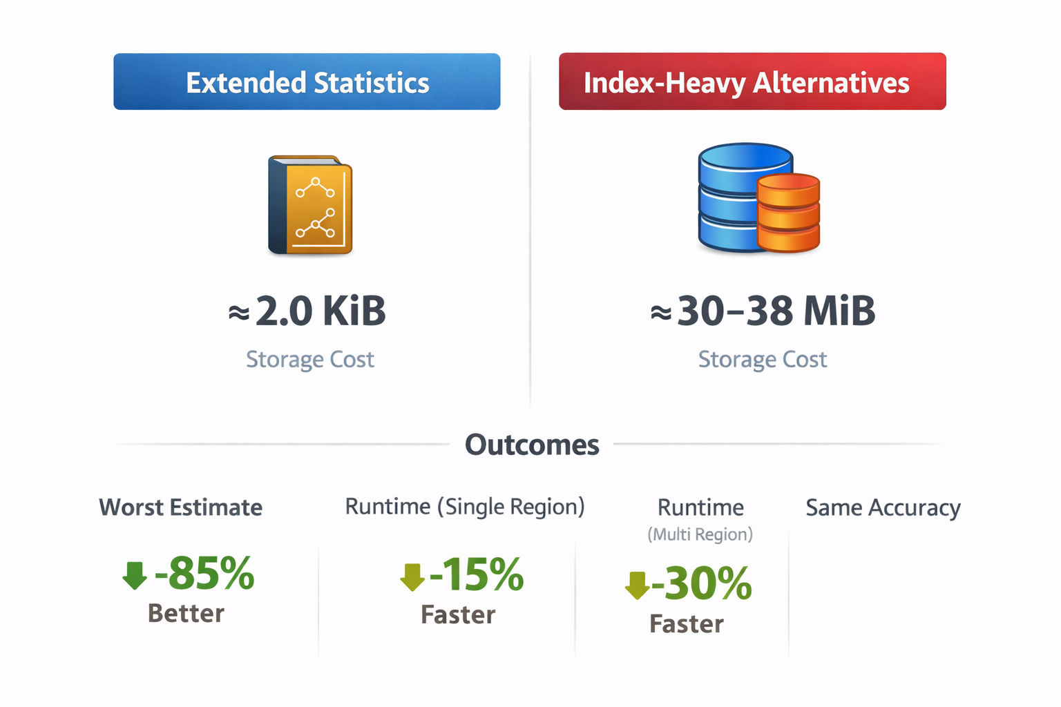
Extended statistics made PostgreSQL much less wrong at the cost of about 2 KiB of metadata, while index-based alternatives required tens of MiB of extra storage and still did not solve the same problem.
Indexes are not useless here. Some absolutely improved access behavior. Some reduced heap work. Some enabled better local execution paths.
But most of them did not solve the planner problem. I’d recommend trying to try combining the two, searching for the best tradeoff between speed and storage cost. But…
Why “Use Both” Did Not Automatically Win
I also tested the obvious question, is combining extended statistics with optimal indexing even better?
Unexpectedly, that did not automatically jump ahead of the individual tests.
Single-region:
- Statistics only: 2,857.896 ms
- Statistics + partial hot-path indexes: 4,876.187 ms
Multi-region:
- Statistics only: 7,289.319 ms
- Statistics + partial hot-path indexes: 8,950.207 ms
Why can that happen?
Because extra indexes do not just add opportunity. They also change the search space.
Once the planner has more selective information, a narrow, query-specific index strategy is not guaranteed to remain the best physical path. Sometimes the combined scenario lands in an awkward middle ground: better beliefs, but worse path selection.
“Use both” is not a law of nature. It is another benchmark question. As I said above, try to combine, not just blindly do both. Indexes and extended statistics influence the planner's decisions and may create mutually exclusive query plans for better or worse.
Practical Caveats
A few caveats are worth being explicit about.
First, extended statistics apply only within a single relation. They do not directly model cross-table correlations.
Second, PostgreSQL still does not use extended statistics directly for join selectivity estimation. That sounds more limiting than it is, because fixing a single-table estimate can still materially change downstream join choices.
Third, not every workload benefits. If your columns are genuinely close to independent, extended statistics may not buy you much.
Fourth, extended statistics don’t replace good query design, useful indexes, partitioning (yes, declarative partitioning is awesome!), sensible memory settings, and a fast storage engine.
They are a planner-information feature, not a universal performance charm.
Finally, the first metric to watch is not always elapsed time. Often, it is estimated quality. If estimates improve dramatically and runtime does not, that still tells you something valuable: the planner model is healthier, and the real bottleneck may now be elsewhere.
When To Reach For CREATE STATISTICS
The practical rule is simple: if a query plan looks wrong, and the wrongness seems tied to multiple columns being filtered or grouped together in a way the planner is modeling badly, think about extended statistics before you immediately build another index.
Good candidates include:
- Highly correlated filtering columns
- Segment-driven dimension attributes
- Group-by workloads where cardinality is obviously off
- Multi-column fanout problems
- Skewed combinations of common values
- Workloads where one bad single-table estimate poisons the rest of the plan
Less good candidates include:
- Queries whose real problem is a missing access path
- Workloads dominated by obvious I/O bottlenecks
- Cases where the columns are actually close to independent
And remember, while they may lower the impact, extended statistics are not a replacement for indexes.
If PostgreSQL is making poor choices due to incorrect row counts, CREATE STATISTICS is often the cheapest way to correct those beliefs. Use EXPLAIN (ANALYZE, VERBOSE, BUFFERS) to verify execution plans. If you see vast discrepancies between estimated and actual row counts, extended statistics may be beneficial.
Prefer Truth Over Tricks
The best thing about CREATE STATISTICS is the reward of understanding the data instead of just piling on more structures.
It forces you to think about how columns relate to each other, how join fanout actually works, and whether the planner’s mental model matches reality. That is less emotionally satisfying than creating a heroic index with a very long name, but it is often more correct.
The benchmark results here do not say “extended statistics always win.” They say something better.
- They made PostgreSQL much less wrong.
- They changed the plan shape in meaningful ways.
- They cost almost nothing to store.
- They often addressed the planner problem more directly than tens of MiB of extra indexes.
The benchmark and the results are on GitHub. You can quickly sign up for our Vela Postgres Sandbox and test the queries yourself.
I also would love to hear about your experiences with extended statistics. As mentioned in the beginning, I never used them in production, and I think I was very wrong. But I’d love to hear from you!
And if you have ever looked at a plan and thought, there is no way this join should be nested three times in a trench coat, extended statistics might be the feature you were actually looking for.